- interpret regression statistics table
- interpret the ANOVA table (often this is skipped)
- interpret regression coefficients table
- test hypothesis of zero slope parameter
- test hypothesis of slope parameter equal to a particular value other than zero
- obtain a confidence interval for slope parameter
- test overall significance of the regressors
- predict Y given values of regressors
- fitted values and residuals from regression line
- other regression output (more details to come)
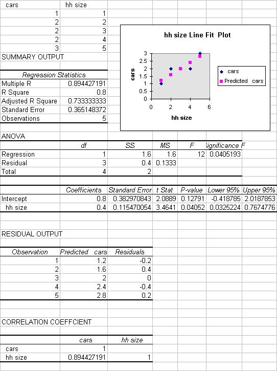
- Excel output for this example.
This handout is the place to go to for statistical inference for two-variable
regression output.
INPUT DATA
The data used are in number of cars per household (Y) and household size (X).
The spreadsheet cells A1:B6 should look like:
| cars | hh size |
| 1 | 1 |
| 2 | 2 |
| 2 | 3 |
| 2 | 4 |
| 3 | 5 |
RUN THE REGRESSION
The population regression model is
y = b1 + b2*x + u
where the error term u has mean 0 and variance sigma-squared.
We wish to estimate the regression line
y = b1 + b2*x
Do this by Tools / Data Analysis / Regression.
A relatively simple form of the command (with labels and line plot) is
| Input Y Range | a1:a6 |
| Input X Range | b1:b6 |
| Labels | Tick |
| Output range | a8 |
| Line Plot | Tick |
and then hit OK.
REGRESSION SUMMARY OUTPUT
There is quite a lot of regression output produced (see end for all the output):
- Regression statistics table
- ANOVA table
- Regression coefficients table.
INTERPRET REGRESSION STATISTICS TABLE
| Explanation | ||
| Multiple R | 0.894427 | R = square root of R^2 |
| R Square | 0.8 | R^2 = coefficient of determination |
| Adjusted R Square | 0.733333 | Adjusted R^2 used if more than one x variable |
| Standard Error | 0.365148 | This is the sample estimate of the st. dev. of the error u |
| Observations | 5 | Number of observations used in the regression (n) |
The above gives the overall goodness-of-fit measures:
R-squared = 0.8
Correlation between y and x is 0.8944 (when squared gives 0.8).
Adjusted R-squared will be discussed later when more than one regressor is
present.
The standard error here refers to the estimated standard deviation of the
error term u.
It is sometimes called the standard error of the regression. It equals sqrt(SSE/(n-k)).
It is not to be confused with the standard error of y itself (from descriptive
statistics) or with the standard errors of the regression coefficients given
below.
INTERPRET ANOVA TABLE
| df | SS | MS | F | Signifiance F | |
| Regression | 1 | 1.6 | 1.6 | 12 | 0.04519 |
| Residual | 3 | 0.4 | 0.133333 | ||
| Total | 4 | 2.0 |
The above ANOVA (analysis of variance) table splits the sum of squares into its components.
Total sums of squares
= Residual (or error) sum of squares + Regression (or explained) sum of squares.
Thus Sum (y_i - ybar)^2 = Sum (y_i - yhat_i)^2 + Sum (yhat_i - ybar)^2.
For example, R-squared = 1 - Residual SS/Total SS = 1 - 0.4/2.0 = 0.8.
The remainder of the ANOVA table is described in more detail in
Excel: Multiple Regression.
INTERPRET REGRESSION COEFFICIENTS TABLE
| Coefficient | St. error | t Stat | P-value | Lower 95% | Upper 95% | |
| Intercept | 0.8 | 0.38297 | 2.089 | 0.1279 | -0.4188 | 2.0188 |
| hh size | 0.4 | 0.11547 | 3.464 | 0.0405 | 0.0325 | 0.7675 |
Let b1 denote the population coefficient of the intercept and b2 the
population coefficient of hh size.
Here we focus on inference on b2, using the row that begins with hh size.
Similar interpretation is given for inference on b1, using the row that begins
with intercept.
The column "Coefficient" gives the least squares estimates of b2.
The column "Standard error" gives the standard errors (i.e.the estimated standard deviation) of the least squares estimate of b2.
The column "t Stat" gives the computed t-statistic for H0: b2 = 0 against Ha:
bj does not equal 0.
This is the coefficient divided by the standard error. It is compared to a t
with (n-k) degrees of freedom where here n = 5and k = 2.
The column "P-value" gives for hh size are for H0: b2 = 0 against Ha: b2 does
not equal 0.
This equals the Pr{|t| > t-Stat}where t is a t-distributed random variable with
n-k degreres of freedom and t-Stat is the computed value of the t-statistic
given is the previous column.
Note that this P-value is for a 2-sided test.
For a 1-sided test divide this P-value by 2 (also checking the sign of the
t-Stat).
The columns "Lower 95%" and "Upper 95%" values define a 95% confidence interval for b2.
A simple summary of the above output is that the fitted line is
y = 0.8+0.4*x
where the slope coefficient has estimated standard error of 0.115, t-statistic of 3.464 and p-value of 0.0405. There are 5 observations and 2 regressors (intercept and x) so we use t(5-2)=t(3).
A measure of the fit of the model is R^2=0.8, which means that 80% of the
variation of y_i around ybar is explained by the regressor x_i. The standard
error of the regression is 0.365148.
TEST HYPOTHESIS OF ZERO SLOPE COEFFICIENT
Test H0: b2 = 0 against Ha: b2 not equal to 0, at significance level alpha = .05.
Reject H0 as from output t2 = 3.464 > t_.025(3) = 3.182 (from tables).
Or reject H0 as from output p-value = 0.0405 < 0.05.
Aside: Excel calculates t2 = b2 / se2 = 0.4/0.11547
and p-value as Pr(|t| > 3.464|t is t(3))
TEST HYPOTHESIS OF ZERO SLOPE COEFFICIENT
Excel automatically gives output to make this test easy.
Consdier test H0: b2 = 0 against Ha: b2 not equal to 0, at significance level alpha = .05.
Using the p-value approach, the p-value given in the output is exactly the
p-value we want.
So p-value = 0.0405. Since p-value is < 0.05 we reject the null hypothesis.
Using the critical value approach, the t-test statistic given in the output
is exactly the t-statistic we want.
So t-statistic = 3.464. Now t_.025(3) = 3.182 from Excel or tables.
Since t-statistic > 3.182 we reject the null hypothesis.
Aside: Excel calculates t2 = b2 / se2 = 0.4/0.11547
and p-value as Pr(|t| > 3.464|t is t(3))
If instead one-sided tests are performed, we need to adjust the above.
For the p-value approach the reported p-value is for a two-sided test and needs
to be halved for a one-sided test.
For the t-statistic approach the reported t-statistic is appropriate but the
critical value is now t_.05(3)=2.353.
Further refinement is needed depending on the direction of the one-tailed test.
See a textbook.
TEST HYPOTHESIS OF SLOPE COEFFICIENT EQUAL TO VALUE OTHER THAN ZERO
For non-zero hypthesized value of the slope parameter we need to .
Suppose we want to test H0: b2=1.0 against H0:b2 not equal to 0.
i.e. that an extra household member means an extra car.
Then t = (b2 - estimated b2) / standard error of estimate
so t = (0.4 - 1.0) / 0.11457 = -5.196.
Using the either the p-value or critical value approach will lead to rejection
of H0 at 5%. See a textbook.
95% CONFIDENCE INTERVAL FOR SLOPE COEFFICIENT
95% confidence interval for slope coefficient is from Excel output (.0325, .7675).
Aside: Excel computes this as
b2 +/- t_.025(3)*seb2
= 0.8 +/- 3.182*0.11547
= 0.8 +/- .367546
= (.0325,.7675).
FITTED VALUES AND RESIDUALS FROM REGRESSION LINE
Fitted values and residuals from the regression line
| y = cars | x = hh size | yhat = 0.8+0.4*x | e = y - yhat |
| 1 | 1 | 1.2 | -.2 |
| 2 | 2 | 1.6 | 0.4 |
| 2 | 3 | 2.0 | 0.0 |
| 2 | 4 | 2.4 | -.4 |
| 3 | 5 | 2.8 | 0.2 |
PREDICTED VALUE OF Y GIVEN X = 4
yhat = b1 + b2*x = 0.8 + 0.4*4 = 2.4.
This is also the predicted value of the conditional mean of y given x=4.
OTHER REGRESSION OUTPUT
Other useful options of the regression command include:
Confidence Level other than 95% gives confidence intervals for b1 and b2 at
level other than 95%.
Line Fit Plots plots the fitted and actual values yhat_i and y_i against x_i.
Discussion of this is still to come.
COMPLETE EXCEL OUTPUT FOR THIS EXERCISE