This page gives information on how to
There is little extra to know beyond regression with one explanatory
variable.
The main addition is the F-test for overall fit.
Here Tools | Data Analysis | Regression is used.
One can also use Excel functions LINEEST and TREND, see Excel: Two Variable
Regression using Excel Functions
DATA
Consider the following data on the number of cars in a household (first
column) and the number of persons in the household (second column).
| 1 | 1 |
| 2 | 2 |
| 2 | 3 |
| 2 | 4 |
| 3 | 5 |
Type the data into cells A1:A5 and cells B1:B5.
Then give headers in a new first row of CARS and HH SIZE to the two columns.
Then create a new variable in cells C2:C6, cubed household size as a regressor,
and give in C1 the heading CUBED HH SIZE. (It turns out that squared hh size has
a coefficient of exactly 0.0 so I use the cube).
The spreadsheet cells A1:C6 should look like:
| CARS | HH SIZE | CUBED HH SIZE |
| 1 | 1 | 1 |
| 2 | 2 | 8 |
| 2 | 3 | 27 |
| 2 | 4 | 64 |
| 3 | 5 | 125 |
RUN THE REGRESSION
The population regression model is
y = b1 + b2*x + b3*z + u
where here z = x^3 and the error term u has mean 0 and variance sigma-squared.
We wish to estimate the regression line
y = b1 + b2*x + b3*z
Do this by Tools / Data Analysis / Regression.
The only change over one-variable regression is to include more than one column
in the Input X Range.
A relatively simple form of the command (with labels) is
| Input Y Range | a1:a6 |
| Input X Range | b1:c6 |
| Labels | Tick |
| Output range | a8 |
and then hit OK.
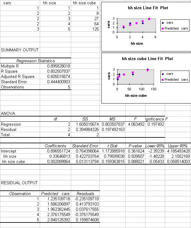
Complete output for this example is given at the bottom.
Here we go through the output in detail, considering both data summary and
statistical inference.
REGRESSION STATISTICS
This is the following output. Of greatest interest is R Square.
| Explanation | ||
| Multiple R | 0.895828 | R = square root of R^2 |
| R Square | 0.802508 | R^2 = coefficient of determination |
| Adjusted R Square | 0.605016 | Adjusted R^2 used if more than one x variable |
| Standard Error | 0.444401 | This is the sample estimate of the st. dev. of the error u |
| Observations | 5 | Number of observations used in the regression (n) |
The above gives the overall goodness-of-fit measures:
R-squared = 0.8025
Correlation between y and y-hat is 0.8958 (when squared gives 0.8).
Adjusted R-squared = R^2 - (1-R^2)*(k-1)/(n-k) = .8025 - .1975*2/2
The standard error here refers to the estimated standard deviation of the
error term u.
It is sometimes called the standard error of the regression. It equals sqrt(SSE/(n-k)).
It is not to be confused with the standard error of y itself (from descriptive
statistics) or with the standard errors of the regression coefficients given
below.
ANOVA
An ANOVA table is given. This is often skipped.
| df | SS | MS | F | Significance F | |
| Regression | 2 | 1.6050 | 0.8025 | 4.0635 | 0.1975 |
| Residual | 2 | 0.3950 | 0.1975 | ||
| Total | 4 | 2.0 |
The above ANOVA (analysis of variance) table splits the sum of squares into its components.
Total sums of squares
= Residual (or error) sum of squares + Regression (or explained) sum of squares.
Thus Sum (y_i - ybar)^2 = Sum (y_i - yhat_i)^2 + Sum (yhat_i - ybar)^2.
The column labeled F gives the overall F-test of H0: b2 = 0 and b3 = 0 versus
Ha: at least one does not equal zero.
Aside: Excel computes F this as:
F = [Regression SS/(k-1)] / [Residual SS/(n-k)] = [1.6050/2] / [.39498/2] =
4.0635.
The column labeled significance F has the associated P-value. Since it is
greater than 0.05 at the 5% siginificance level we do not reject H0.
KEY REGRESSION OUTPUT
The regression output of most interest is the following table of coefficients
and associated output:
| Coefficient | St. error | t Stat | P-value | Lower 95% | Upper 95% | |
| Intercept | 0.89655 | 0.76440 | 1.1729 | 0.3616 | -2.3924 | 4.1855 |
| HH SIZE | 0.33647 | 0.42270 | 0.7960 | 0.5095 | -1.4823 | 2.1552 |
| CUBED HH SIZE | 0.00209 | 0.01311 | 0.1594 | 0.8880 | -0.0543 | 0.0585 |
Let bj denote the population coefficient of the jth regressor (intercept, HH SIZE and CUBED HH SIZE).
Then
A simple summary of the above output is that the fitted line is
y = 0.8966 + 0.3365*x + 0.0021*z
TEST OF STATISTICAL SIGNIFICANCE
The coefficient of HH SIZE has estimated standard error of 0.4227,
t-statistic of 0.7960 and p-value of 0.5095.
It is therefore statistically insignificant at 5%.
The coefficient of CUBED HH SIZE has estimated standard error of 0.0131,
t-statistic of 0.1594 and p-value of 0.8880.
It is therefore statistically insignificant at 5%.
There are 5 observations and 3 regressors (intercept and x) so we use
t(5-3)=t(2).
GOODNESS OF FIT
A measure of the fit of the model is R^2=0.803, which means that 80.3%
of the variation of y_i around ybar is explained by the regressor x_i.
The standard error of the regression is 0.365148.
TEST HYPOTHESIS ON A REGRESSION PARAMETER
Here we consider test of zero slope parameter.
This will reproduce the results for statistical significance. We could change to
testing other values.
Example: Test H0: b2 = 0 against Ha: b2 not equal to 0, at significance level alpha = .05.
Do not reject H0 as p-value = 0.5095 > 0.05.
Equivalently, so not reject H0 as t2 = 0.7960 < t_.025(2) = 4.303 (from tables
where here n-k = 4-3 = 2).
Aside: Excel calculates t2 = b2 / se2 = 0.3365/0.4227
and p-value as Pr(|t| > 0.5095 | t is t(2))
CONFIDENCE INTERVAL FOR REGRESSION PARAMETER
95% confidence interval for coefficient of HH SIZE is from Excel output
(-1.4823, 2.1552).
OVERALL TEST OF SIGNIFICANCE OF THE REGRESSION PARAMETERS
We test H0: b2 = 0 and b3 = 0 against Ha: at least one of b2 and b3 is not
equal to 0.
From the ANOVA table the F-test statistic is 4.0635 with p-value of 0.1975.
Since the p-value is not less than 0.05 we do not reject the null hypothesis
that the regression parameters are zero at significance level 5%.
Conclude that the parameters are jointly statistically insignificant at
significance level 5%.
PREDICTED VALUE OF Y GIVEN REGRESSORS
Consider case where x = 4 in which case z = x^3 = 4^3 = 64.
yhat = b1 + b2*x + b3*z = 0.88966 + 0.3365*4 + 0.0021*64 = 2.37006.
This is also the predicted value of the conditional mean of y given x=4 and
z=64.
OTHER REGRESSION OUTPUT
Other useful options of the regression command include:
Confidence Level other than 95% gives confidence intervals for b1 and b2 at
level other than 95%.
Line Fit Plots plots the fitted and actual values yhat_i and y_i against x_i.
These are similar to what is discussed in bivariate regression.
LIMITATIONS
Excel will only permit up to 16 regressors.
Excel requires that all the regressor variables be in adjoining columns.
You may need to move columns to ensure this.
e.g. If the regressors are in columns b and d you need to copy at least one of
columns b and d so that they are adjacent to each other.
EXCEL OUTPUT FOR THIS EXERCISE