New Page 1

MGS3100: Forecasting & Quality Management

Sample Questions for Exam 2

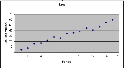
Consider the time series below with 15 observations. Two types of forecasts are shown – 4 period moving average and Simple Exponential Smoothing with an alpha of 0.5. Fill in the blanks where appropriate and calculate the BIAS, MAD, and Standard Error for both methods.

							alpha=	0.5
		4 period		Abs	Error	Exponential		Abs	Error
Period	Sales	Average	Error	Error	Squared	Smoothing	Error	Error	Squared
1	5
2	8
3	16
4	17
5	22					14.13	7.88	7.88	62.02
6	28					18.06	9.94	9.94	98.75
7	26	20.75	5.25	5.25	27.56	23.03	2.97	2.97	8.81
8	35	23.25	11.75	11.75	138.06	24.52	10.48	10.48	109.92
9	36	27.75	8.25	8.25	68.06	29.76	6.24	6.24	38.96
10	39	31.25	7.75	7.75	60.06	32.88	6.12	6.12	37.47
11	44	34.00	10.00	10.00	100.00	35.94	8.06	8.06	64.97
12	41	38.50	2.50	2.50	6.25	39.97	1.03	1.03	1.06
13	47	40.00	7.00	7.00	49.00	40.48	6.52	6.52	42.45
14	55	42.75	12.25	12.25	150.06	43.74	11.26	11.26	126.73
15	60	46.75	13.25	13.25	175.56	49.37	10.63	10.63	112.97

Summarize your computations in the table below.

BIAS

MAD

Standard Error

4 Period

Average

Exponential Smoothing

1. Interpret the BIAS and MAD.

2. Based on the above table, which is the better forecast? Why?

3. Use the better of the two methods to forecast sales for the 16^th period.

4. Above is a scatter plot of the same data. What method does this indicate as the best one to use for forecasting?

5. Write down the estimated simple regression function (visual estimate) from the above graph.

SUMMARY OUTPUT

Regression Statistics
Multiple R	0.9882
R Square

Standard Error
Observations	15

ANOVA
	df	SS	MS	F	Significance F
Regression	1	3686.629		542.736	0.000
Residual	13	88.305
Total	14	3774.933

	Coefficients	Standard Error	t Stat	P-value	Lower 95%	Upper 95%	Lower 95.0%	Upper 95.0%
Intercept	2.9048	1.4161	2.0512	0.0610	-0.1546	5.9641	-0.1546	5.9641
Period	3.6286	0.1558	23.2967	0.0000	3.2921	3.9651	3.2921	3.9651



RESIDUAL OUTPUT

Observation	Predicted Sales	Residuals
1	6.5333	-1.5333
2	10.1619	-2.1619
3	13.7905	2.2095
4	17.4190	-0.4190
5	21.0476	0.9524
6	24.6762	3.3238
7	28.3048	-2.3048
8	31.9333	3.0667
9	35.5619	0.4381
10	39.1905	-0.1905
11	42.8190	1.1810
12	46.4476	-5.4476
13	50.0762	-3.0762
14	53.7048	1.2952
15	57.3333	2.6667

Consider the regression output shown above for the same data.

6. What is the regression equation?

7. Forecast the sales for period 16.

8. Calculate BIAS, MAD, and Std. Error for the regression.

9. Based on the above criteria, how does this method fare compared to the heuristic methods?

10. Calculate R-squared and interpret the value.

11. Is the regression statistically significant?

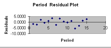
12. Does the Residual plot below suggest that some other regression function must be used instead of the simple linear model?

13. What is a seasonal index? What would a seasonal index of 1.25 mean?

14. Is the BIAS for a forecast using Log Y regression equal to 0?

15. If the forecasted log Y is 6.34, what is the forecasted value of Y?

16. If the forecasted deseasonalized Y for Quarter 1 is 34, what is the forecasted Y for that quarter if the seasonal indices are as follows:

Quarter1	Quarter2	Quarter3	Quarter4
missing	1.2	0.9	1.1